Hello Everyone!
For the first project conducted exclusively for this blog, I wanted to work on something near and dear to my heart. Cats.

Where did this data come from?
If you haven't heard, https://toolbox.google.com/datasetsearch is awesome.
As I often do when exposed to a new tool, I typed in "cat" to see what would happen.
In so doing, I was rewarded with the Cat Personality Dataset from https://data.unisa.edu.au/Dataset.aspx?DatasetID=271178
Published in March 2018, this is a FIFTY-TWO item dataset quantifying the personality of 2802 cats.
They are from Australia and New Zealand, but I am going to assume no major differences at this point.
I should also point out that each entry is a 1-7 scale filled out by the owner, not that cat. So these cat owners saw something similar to "Is your cat Erratic? (rate 1-7)", and did that 51 other times.
What sort of questions can we answer?
I wanted to understand what types of cats exist in this data set, and so, potentially, the world.
Every cat is special, and the number of possible combinations in this data set is 7^52 or 88,124,000,000,000,016,384,184,968,936,160,080,432,408,840 possible cats. This isn't useful at all.
How can I reduce this number to something I can get my brain around?
The answer is clustering. This is a form of unsupervised learning in which we apply an algorithm to data in order to figure out which features (cat attributes, in this case) group together, and which ones distinguish different categories of cats.
Alternatives exist, such as PCA, or k-means++, but this is a fine starting point.
Given the attributes included in the survey, it seems CERTAIN that some will group together ("Gentle" and "Calm") whereas others will be quite distinct ("Predictable" and "Erratic")
import pandas as pd
import numpy as np
from pathlib import Path
from sklearn.cluster import KMeans
import matplotlib.pyplot as plt
from sklearn import metrics
from scipy.spatial.distance import cdist
# loading the data
data_folder = Path("E:/Downloads")
file_to_open = data_folder / "Cat_personality_data.csv"
df = pd.read_csv(file_to_open)
df.head()
| Personality1_Vigilant | Personality2_Stable | Personality3_Bold | Personality4_Clumsy | Personality5_Defiant | Personality6_Gentle | Personality7_Constrained | Personality8_Inquisitive | Personality9_Inventive | Personality10_Irritable | ... | Personality45_Decisive | Personality46_Self_assured | Personality47_Anxious | Personality48_Trusting | Personality49_Active | Personality50_Cooperative | Personality51_Shy | Personality52_Eccentric | Country | Cat_sex | |
|---|---|---|---|---|---|---|---|---|---|---|---|---|---|---|---|---|---|---|---|---|---|
| 0 | 6 | 5 | 7 | 5 | 5 | 6 | 1 | 5 | 4 | 3 | ... | 4 | 6 | 4 | 5 | 7 | 2 | 2 | 4 | NewZealand | Male |
| 1 | 7 | 3 | 4 | 1 | 7 | 7 | 3 | 4 | 3 | 2 | ... | 4 | 3 | 6 | 6 | 1 | 6 | 2 | 5 | NewZealand | Female |
| 2 | 7 | 5 | 7 | 1 | 2 | 3 | 3 | 7 | 7 | 2 | ... | 7 | 6 | 3 | 4 | 7 | 2 | 3 | 4 | Australia | Male |
| 3 | 7 | 4 | 1 | 1 | 7 | 2 | 7 | 1 | 3 | 7 | ... | 5 | 3 | 3 | 2 | 2 | 2 | 6 | 2 | Australia | Female |
| 4 | 5 | 7 | 7 | 1 | 4 | 7 | 7 | 4 | 4 | 1 | ... | 5 | 7 | 1 | 7 | 7 | 6 | 2 | 7 | Australia | Male |
5 rows × 54 columns
# cleaning up names
names = []
for i in df.columns[0:1]:
    #print(i[14:])
    names.append(i[14:])
for i in df.columns[1:9]:
    #print(i[13:])
    names.append(i[13:])
for i in df.columns[9:-2]:
    #print(i[14:])
    names.append(i[14:])
for i in df.columns[-2:]:
    #print(i)
    names.append(i)
df.columns=names
# visualizing the results
df.head()
| Vigilant | Stable | Bold | Clumsy | Defiant | Gentle | Constrained | Inquisitive | Inventive | Irritable | ... | Decisive | Self_assured | Anxious | Trusting | Active | Cooperative | Shy | Eccentric | Country | Cat_sex | |
|---|---|---|---|---|---|---|---|---|---|---|---|---|---|---|---|---|---|---|---|---|---|
| 0 | 6 | 5 | 7 | 5 | 5 | 6 | 1 | 5 | 4 | 3 | ... | 4 | 6 | 4 | 5 | 7 | 2 | 2 | 4 | NewZealand | Male |
| 1 | 7 | 3 | 4 | 1 | 7 | 7 | 3 | 4 | 3 | 2 | ... | 4 | 3 | 6 | 6 | 1 | 6 | 2 | 5 | NewZealand | Female |
| 2 | 7 | 5 | 7 | 1 | 2 | 3 | 3 | 7 | 7 | 2 | ... | 7 | 6 | 3 | 4 | 7 | 2 | 3 | 4 | Australia | Male |
| 3 | 7 | 4 | 1 | 1 | 7 | 2 | 7 | 1 | 3 | 7 | ... | 5 | 3 | 3 | 2 | 2 | 2 | 6 | 2 | Australia | Female |
| 4 | 5 | 7 | 7 | 1 | 4 | 7 | 7 | 4 | 4 | 1 | ... | 5 | 7 | 1 | 7 | 7 | 6 | 2 | 7 | Australia | Male |
5 rows × 54 columns
df=df.iloc[:,:-2] # we drop gender and nationality for now
# entering it into k-means clustering
X = df.values
kmeans = KMeans(
    n_clusters=5,
    random_state=0).fit(X)
kmeans.labels_ #these are the clusters it came up with
array([2, 3, 2, ..., 0, 4, 4])
df['cluster']=kmeans.labels_
So, we have 5 clusters of cats. Is that the right number?
For this, I turned to what's known as a "Scree Plot". AKA, trying a bunch of different numbers.
It's worth noting that I ran this several times as, in k-means, you can get a sub-optimal clustering based on initial conditions}.
# thanks to:
# https://pythonprogramminglanguage.com/kmeans-elbow-method/
# k means determine k
distortions = []
K = range(1,20)
for k in K:
    kmeanModel = KMeans(n_clusters=k).fit(X)
    kmeanModel.fit(X)
    distortions.append(sum(np.min(cdist(X, kmeanModel.cluster_centers_, 'euclidean'), axis=1)) / X.shape[0])
# Plot the elbow
plt.plot(K, distortions, 'bx-')
plt.xlabel('k')
plt.ylabel('Distortion')
plt.title('The Elbow Method showing the optimal k')
plt.show()
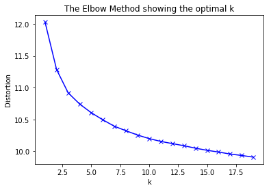
This indicates that while our clusters fit better and better as we assert that there are more and more different types of cats, the big gains are made at k = 10, or maybe even k=7.
One of the advantages of kmeans is that it was trivial to work in 52-dimensional space. Now, however, that makes visualization a bit mind boggling. What we can do is examine the weakest and strongest average attributes for each cluster.
# repeating what we did above with clusters = 7
X = df.values
kmeans = KMeans(
    n_clusters=7,
    random_state=0).fit(X)
df['cluster']=kmeans.labels_
cluster_attributes=df.groupby(['cluster']).mean()
zero_cluster=cluster_attributes[cluster_attributes.index==0].T
# Get top 3 and bottom 3 for one cluster
zero_cluster=cluster_attributes[cluster_attributes.index==0].T
sorted_zero_cluster=zero_cluster.sort_values(by=0)
top_sorted_zero_cluster=sorted_zero_cluster.iloc[[49,50,51]]
bottom_sorted_zero_cluster=sorted_zero_cluster.iloc[[0,1,2]]
bottom_sorted_curr_cluster.index.tolist()
['Aggressive_to_people', 'Irritable', 'Tense']
bottom_sorted_zero_cluster
| cluster | 0 |
|---|---|
| Aggressive_to_people | 1.459290 |
| Clumsy | 1.812109 |
| Erratic | 2.008351 |
# Repeat for each cluster:
cluster_output = []
top_attributes = []
bot_attributes = []
for i in range(7):
    curr_cluster=cluster_attributes[cluster_attributes.index==i].T
    sorted_curr_cluster=curr_cluster.sort_values(by=i)
    top_sorted_curr_cluster=sorted_curr_cluster.iloc[[49,50,51]]
    bottom_sorted_curr_cluster=sorted_curr_cluster.iloc[[0,1,2]]
    cluster_output.append([i,i,i])
    top_attributes.append(top_sorted_curr_cluster.index.tolist())
    bot_attributes.append(bottom_sorted_curr_cluster.index.tolist())
    #print("cluster ",i," top traits:")
    #print(top_sorted_curr_cluster)
    #print("cluster ",i," bottom traits:")
    #print(bottom_sorted_curr_cluster)
top_df = pd.DataFrame(data=top_attributes, columns=['highest', 'second highest', 'third highest'])
bot_df = pd.DataFrame(data=bot_attributes,columns=['lowest', 'second lowest', 'third lowest'])
results_df=top_df.join(bot_df, rsuffix='_bot')
results_df.T
| 0 | 1 | 2 | 3 | 4 | 5 | 6 | |
|---|---|---|---|---|---|---|---|
| highest | Affectionate | Friendly_to_people | Smart | Inquisitive | Predictable | Friendly_to_people | Friendly_to_people |
| second highest | Vigilant | Playful | Suspicious | Smart | Insecure | Affectionate | Gentle |
| third highest | Smart | Affectionate | Vigilant | Self_assured | Suspicious | Gentle | Affectionate |
| lowest | Aggressive_to_people | Aggressive_to_people | Clumsy | Clumsy | Aggressive_to_people | Aggressive_to_people | Aggressive_to_people |
| second lowest | Clumsy | Irritable | Friendly_other_cats | Submissive | Bullying | Erratic | Irritable |
| third lowest | Erratic | Fearful_of_people | Submissive | Aggressive_to_people | Bold | Fearful_of_people | Tense |
What do we think of these?
First, considering the highest rated attribute of each cluster. Friendly to people is higest rated in 3 of our 7 categories. (1, 5, and 6) While it makes sense that people have cats that love them, I wonder what makes those categories different? Affectionate ranks very highly in those categories too.
For those same categories, Fearful_of_people is low. Makes sense.

More interesting perhaps, are the "smart cats". The ravenclaws, if you will.
Cluster 0 is still affectionate, but is also rated highly for Vigilance and Smarts.
Cluster 2 has actually lost affection as one of their top attributes, and has "Suspicious"
Cluster 3 is highest rated as inquisitive, as well as self assured.

Finally, poor cluster 4. They're Predictable, Insecure, and Suspicious.
So it looks like we have some interesting information, but that this data probably needs a bit more massaging. To follow up on what we've done here, let's just see how widely distributed our clusters are.
df.groupby('cluster').count()
| Vigilant | Stable | Bold | Clumsy | Defiant | Gentle | Constrained | Inquisitive | Inventive | Irritable | ... | Playful | Vocal | Decisive | Self_assured | Anxious | Trusting | Active | Cooperative | Shy | Eccentric | |
|---|---|---|---|---|---|---|---|---|---|---|---|---|---|---|---|---|---|---|---|---|---|
| cluster | |||||||||||||||||||||
| 0 | 479 | 479 | 479 | 479 | 479 | 479 | 479 | 479 | 479 | 479 | ... | 479 | 479 | 479 | 479 | 479 | 479 | 479 | 479 | 479 | 479 |
| 1 | 317 | 317 | 317 | 317 | 317 | 317 | 317 | 317 | 317 | 317 | ... | 317 | 317 | 317 | 317 | 317 | 317 | 317 | 317 | 317 | 317 |
| 2 | 476 | 476 | 476 | 476 | 476 | 476 | 476 | 476 | 476 | 476 | ... | 476 | 476 | 476 | 476 | 476 | 476 | 476 | 476 | 476 | 476 |
| 3 | 473 | 473 | 473 | 473 | 473 | 473 | 473 | 473 | 473 | 473 | ... | 473 | 473 | 473 | 473 | 473 | 473 | 473 | 473 | 473 | 473 |
| 4 | 349 | 349 | 349 | 349 | 349 | 349 | 349 | 349 | 349 | 349 | ... | 349 | 349 | 349 | 349 | 349 | 349 | 349 | 349 | 349 | 349 |
| 5 | 259 | 259 | 259 | 259 | 259 | 259 | 259 | 259 | 259 | 259 | ... | 259 | 259 | 259 | 259 | 259 | 259 | 259 | 259 | 259 | 259 |
| 6 | 449 | 449 | 449 | 449 | 449 | 449 | 449 | 449 | 449 | 449 | ... | 449 | 449 | 449 | 449 | 449 | 449 | 449 | 449 | 449 | 449 |
7 rows × 52 columns
Pretty good distribution. Group 5 is the least with 259 cats, but most have around 350-450.
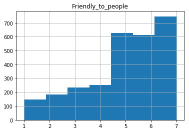
Finally, I want to investigate the distribution of some of these common groups along different clusters.
#all cats included
df.loc[:,['Friendly_to_people']].hist(bins=7)
array([[<matplotlib.axes._subplots.AxesSubplot object at 0x00000000159E7358>]],
      dtype=object)
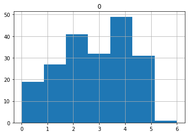
# just one of the friendlies
one=df[df.cluster==1]
one.loc[:,['Friendly_to_people']].hist(bins=7)
array([[<matplotlib.axes._subplots.AxesSubplot object at 0x0000000015D74748>]],
      dtype=object)
# the insecure cats
one=df[df.cluster==4]
one.loc[:,['Friendly_to_people']].hist(bins=7)
array([[<matplotlib.axes._subplots.AxesSubplot object at 0x0000000015DB6828>]],
      dtype=object)
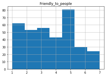
There's a lot more to do here, including PCA and visualization to get an idea of how good the separation is here, but I'm out of time. Gotta go feed my cat.
Tentative findings: - There's about 7 types of cats. - Four flavors of friendly cat. - Two Flavors of smart cat. - One Flavor of scaredy cat.