Punch Classification
As part of my Insight Data Science fellowship, I had the opportunity to work with a startup that was working on a fascinating problem: How to translate three dimensional human movement into something quantifiable. Something we could apply models to to understand.
Specifically, this startup was working on classifying the kinds of punches you would see in boxing into 4 types:

The issue was that they were achieving a limited level of accuracy. Some punches were being misclassified. This was important to their business, as their goal was to give users a strong sense of feedback whenever they threw a punch. If you wanted to see how many jabs you could do in a minute, you wouldn't want to look at your app and see that some of your jabs had been interpreted as uppercuts.
So, my goal was to improve classification accuracy on all 4 types of punches.
How do we tackle this problem?
- Get the data.
- Check for data quality.
- Get a model running.
- Understand what the model is doing.
- Improve the model.
Easy, right?
Getting the data
The first thing I did upon recieving the data was convert the csvs into sql databases. This makes it, in my opinion, much easier to clean and explore. As an added bonus, this means your original data is still just sitting as a csv, and you are free to modify your sql tables as you see fit.
# accessing the data
import psycopg2
import os
import pandas as pd
import matplotlib.pyplot as plt
#get the connection to sql established
dbname = 'punch_db'
username = 'rcphillips'
pswd = 'or1gami4' #anonymity
engine = psycopg2.connect(database = dbname, user = username, host='localhost', password=pswd)
# connection to SQL established. Getting the data into pandas
sql_query = """
SELECT *
FROM puncher_info LEFT JOIN all_punches
ON filename = file
"""
df=pd.read_sql_query(sql_query,engine)
df=df.drop(['name'], axis=1) #anonymity
#did it work?
df.head()
| index | date | filename | impact | side | type | index | xtrans | ytrans | ztrans | xrot | yrot | zrot | file | |
|---|---|---|---|---|---|---|---|---|---|---|---|---|---|---|
| 0 | 0 | 2016-06-07 02:35:01 | 0 | Bag | Right | Hook | 0 | 1537 | 765 | 1216 | 29 | -57 | -98 | 0 |
| 1 | 0 | 2016-06-07 02:35:01 | 0 | Bag | Right | Hook | 1 | 1525 | 772 | 1218 | 43 | -59 | -94 | 0 |
| 2 | 0 | 2016-06-07 02:35:01 | 0 | Bag | Right | Hook | 2 | 1535 | 769 | 1217 | 56 | -61 | -88 | 0 |
| 3 | 0 | 2016-06-07 02:35:01 | 0 | Bag | Right | Hook | 3 | 1545 | 780 | 1224 | 66 | -64 | -87 | 0 |
| 4 | 0 | 2016-06-07 02:35:01 | 0 | Bag | Right | Hook | 4 | 1552 | 787 | 1226 | 68 | -72 | -86 | 0 |
Whenever you come across a dataset, it's essential to ask yourself how it was created. In this case, I had direct access to the people that gathered it.
They told me that they had developed a small device that was inserted into boxers' gloves. It contained a gyroscope, which output information about rotation in space, as well as an accelerometer, which output information about translation (movement) in space.
These two measurements were gathered in three dimensions: x, y and z.
That's how I ended up with the six major features that would describe the spatial position of punches: - xtrans : movement from close to the body to far away from the body. - ytrans : movement from left to right. - ztrans : movement from above to below. - xrot : rotation in the x dimension. - yrot : rotation in the y dimension. - zrot : rotation in the z dimension.
The crucial feature in any machine learning project, the labels, were gathered in the following way:
The members of the startup, or some of their profession boxing supporters, would wear the device, go into the gym, and "do a couple hundred hooks" or "do a couple hundred uppercuts".
The data, in these six dimensions, would come off in a continual stream from the device. This was then "cut up" into individual punches in an automated fashion, by looking for sudden deceleration in x-translation. This is what you would observe if the fist had a sudden impact with something.
It's important to note that the model can do no better than what information you give it. Therefore, if this is how you get your training data, anything with a sudden deceleration will be "turned into a punch". That should be fine most of the time, but if you reach down to pick up a water bottle, you will still have that sudden deceleration in x.
If that motion looks very different from a typical jab, but it is labeled 'jab', the model isn't going to stop you.
Checking this by hand can be bothersome too, given that we have how many examples of each punch?
#now, do that for all punches of a particular type
sql_query = """
SELECT type,
       COUNT(DISTINCT file) as num_punches
FROM puncher_info LEFT JOIN all_punches
ON filename = file
GROUP BY 1
"""
df=pd.read_sql_query(sql_query,engine)
df
| type | num_punches | |
|---|---|---|
| 0 | Block | 1099 |
| 1 | Cross | 1561 |
| 2 | Hook | 1227 |
| 3 | Jab | 1628 |
| 4 | Upper | 536 |
With thousands of datapoints, it's going to be impossible to check it all by hand. I'll be getting to how you can remove abnormal data using anomaly detection, but before I do that, I'll need to create a model to convert these million datapoints into something interpretable.
Get a model running.
When I started looking at this dataset, I tried a variety of models.
The reasons I selected random forest are: - It's easy to set up, so I could start understanding where the classification is failing. - It can capture non-linear relationships between features and labels.
from sklearn.ensemble import RandomForestClassifier
The next question for me was what features would be predictive of the outcomes. We have the amount of movement and rotation in 3 dimensions, but it comes off of the device one thousand times per second.
My goal here was not maximum precision, I just wanted to get to a point where I could understand the misclassifications, so I did the simplest thing I could think of: sum up all the features, per punch.
sql_query = """
SELECT sum(xrot) AS sum_x_rot,
sum(yrot) AS sum_y_rot,
sum(zrot) AS sum_z_rot, file AS rotfile
FROM all_punches
GROUP BY file
"""
df=pd.read_sql_query(sql_query,engine)
df.head()
| sum_x_rot | sum_y_rot | sum_z_rot | rotfile | |
|---|---|---|---|---|
| 0 | -171947.0 | -208979.0 | -86385.0 | 251 |
| 1 | -48981.0 | 74607.0 | 15173.0 | 2848 |
| 2 | -1817.0 | 36412.0 | -11476.0 | 3565 |
| 3 | -134994.0 | 17623.0 | 94362.0 | 2026 |
| 4 | -756.0 | 44930.0 | -6015.0 | 3028 |
I then sent these new features to sql, so I could join them to my existing set of features.
#df.to_sql('all_punches_sum_rot', engine, if_exists = "replace")
#joining aggregate stats to previous df
sql_query = """
SELECT *
FROM all_punches_sum_trans RIGHT JOIN puncher_info
ON file = filename
JOIN all_punches_sum_rot ON file = rotfile
"""
df=pd.read_sql_query(sql_query,engine)
df=df.drop(['name'],axis=1)
df.head()
| index | sum_x_trans | sum_y_trans | sum_z_trans | file | index | date | filename | impact | side | type | index | sum_x_rot | sum_y_rot | sum_z_rot | rotfile | |
|---|---|---|---|---|---|---|---|---|---|---|---|---|---|---|---|---|
| 0 | 107 | 221289.0 | 432786.0 | 150131.0 | 0 | 0 | 2016-06-07 02:35:01 | 0 | Bag | Right | Hook | 107 | -6330.0 | 72822.0 | 136471.0 | 0 |
| 1 | 4372 | 115426.0 | 537033.0 | 290597.0 | 1 | 1 | 2016-06-07 02:35:01 | 1 | Bag | Right | Hook | 4372 | -67156.0 | 69739.0 | 151065.0 | 1 |
| 2 | 5439 | 309867.0 | 213446.0 | 141969.0 | 2 | 2 | 2016-06-07 02:35:01 | 2 | Bag | Right | Hook | 5439 | -33095.0 | 63464.0 | 51166.0 | 2 |
| 3 | 2870 | 306892.0 | 143158.0 | 186782.0 | 3 | 3 | 2016-06-07 02:35:01 | 3 | Bag | Right | Hook | 2870 | -8160.0 | 90687.0 | 98187.0 | 3 |
| 4 | 2782 | 300702.0 | 98481.0 | 133845.0 | 4 | 4 | 2016-06-07 02:35:01 | 4 | Bag | Right | Hook | 2782 | 29462.0 | 84181.0 | 84729.0 | 4 |
Is this going to work? Are our classes actually seperated along this feature? For that, we can do a quick scatterplot.
#defining new columns based on existing ones
matchlist={"Hook":"blue","Upper":"black","Jab":"cyan","Cross":"yellow","Block":"red"}

mylist=list(df.type.values)
colors = list(map(lambda key: matchlist[key], mylist))
df['colors']=colors
#Plotting the data, post-analysis.
%matplotlib inline
fig = plt.figure()
#fig.set_size_inches((10,10))
#ax = plt.axes(projection = '3d')


myplot=plt.scatter(df['sum_x_trans'],df['sum_y_trans'],c=df['colors'])
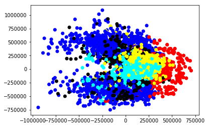
Great! We have some clearly distinct groups. Yes, there's a lot of overlap, but this is just one feature. As we add in additional features, we wil lbe able to make more clean separations.
With those simple features, it's time to test out a model.
# identify labels
y = df['type']
X = df[['sum_x_trans', 'sum_y_trans','sum_z_trans','sum_x_rot', 'sum_y_rot','sum_z_rot']]
model = RandomForestClassifier()
model = model.fit(X, y)
model
RandomForestClassifier(bootstrap=True, class_weight=None, criterion='gini',
            max_depth=None, max_features='auto', max_leaf_nodes=None,
            min_impurity_split=1e-07, min_samples_leaf=1,
            min_samples_split=2, min_weight_fraction_leaf=0.0,
            n_estimators=10, n_jobs=1, oob_score=False, random_state=None,
            verbose=0, warm_start=False)
The model has been initialized. The next step is to randomly remove part of our data, and attempt to use the remaining data to train the model. This means we'll be attempting to learn the relationships between the predictive features and the labels with our "training data". We will then use the model to predict the data we did not use to train. This is our "testing data".
Conveniently, sklearn will split our data into these groups for us.
from sklearn.cross_validation import train_test_split
/Users/rcphillips/anaconda3/lib/python3.5/site-packages/sklearn/cross_validation.py:44: DeprecationWarning: This module was deprecated in version 0.18 in favor of the model_selection module into which all the refactored classes and functions are moved. Also note that the interface of the new CV iterators are different from that of this module. This module will be removed in 0.20.
  "This module will be removed in 0.20.", DeprecationWarning)
X_train, X_test, y_train, y_test = train_test_split(X, y, test_size=0.3)
print(len(y_train))
print(len(y_test))
4235
1816
We have 30% of our data in our test group, and 60% in our training group. Let's get learning.
model.fit(X_train, y_train)
RandomForestClassifier(bootstrap=True, class_weight=None, criterion='gini',
            max_depth=None, max_features='auto', max_leaf_nodes=None,
            min_impurity_split=1e-07, min_samples_leaf=1,
            min_samples_split=2, min_weight_fraction_leaf=0.0,
            n_estimators=10, n_jobs=1, oob_score=False, random_state=None,
            verbose=0, warm_start=False)
So how did we do?
model.score(X_train, y_train)
0.9938606847697756
That may look great, but keep in mind, that's the accuracy for our training data. That's how good the model does at predicting (giving the correct class in response to predictive feature inputs), for examples it's seen before. What about for examples it hasn't seen before? For that, we need to check the performance on the test data.
(I should mention, if you DO have poor training scores, that likely indicates your model is inappropriate for the problem you're trying to solve, or your data needs to be altered in some way. In any case, don't proceed if your training score is below 50% at a minimum)
model.score(X_test, y_test)
0.8133259911894273
Alright! Lower, but not so low that the relationships are not generalizing at all. We want to be sure that we're not just picking up on peculiarities from this test train split, and we want to use all our data, so for that we'll do cross-validation.
from sklearn.cross_validation import cross_val_score
scores = cross_val_score(RandomForestClassifier(), X, y, scoring ='accuracy', cv=10)
scores.mean()
0.739900472616628
That's a bit surprising. It appears we got lucky on our first split. Of course, we should always be looking out for the worst case scenario, because that's what's going to give us trouble in the real world. So let's see how we can improve from here.
Improving the model.
There's a few things we can do.
1) We can tune hyperparameters.
2) We can investigate errors.
Hyperparameter Tuning
Hyperparameter tuning is pretty quick, and gives me a chance to explain the model.
The help file for RandomForestClassifier is quite extensive, and the entry in The Elements of Statistical Learning is even longer, so I will very briefly summarize.
In a random forest model, we use our features to split the data into different groups. We do this repeatedly, resulting in a "tree" of decision points. So, for instance: examples with less than 50 sum_x_trans will be called "group 1" while examples with greater than 50 sum_x_trans will be called "group 2".
The next decision could be: of examples from group 1, those with greater than 50 sum_y_trans will be called "hook" while those with less than 50 sum_y_trans will be called "not hook"
I'm making up these numbers, but its important to note that each split can occur using a different predictive feature.
These splits occur repeatedly until you reach a "minimum_leaf_size". A collection of examples at the bottom of each series of decisions.
The model makes these decisions in order to minimize the amount of different categories in each of these leaves.
What makes random forest a forest is that you have many of these trees, created from different subsets of the data.
What makes random forest random is that prior to each split, you limit the number of predictive features available for future splits, at random.
Doesn't limiting your model's access to information reduce its predictions? No. Because you make so many different trees, and within each of those, so many different splits are made, all the information is used. But this means that your model will explore lots of different possible splits, under lots of different conditions. In this way, you more thoroughly explore the relationship between predictive features and outcome.
Finally, at the end, you "tally the votes" from each tree, for each sample.
The class of punch with the highest output is our model's prediction for that example. This is compared with the label that we know from our data in order to compute the accuracy.
So from that long-winded explanation, what hyperparameters can we tune?
- number of trees
- minimum leaf size
- number of features excluded from each split decision
How we actually do this is easy. We input the appropriate arguments to our model when we initialize it, and then observe the results.
scores = cross_val_score(RandomForestClassifier(n_estimators=50, #the number of trees we'll be using
                                               min_samples_leaf=4, #the minimum size of leaf node
                                               max_features=2 #the number of features considered for a split (out of six)
                                               ), X, y, scoring ='accuracy', cv=10)
scores.mean()
0.7664768482939764
scores = cross_val_score(RandomForestClassifier(n_estimators=200, #the number of trees we'll be using
                                               min_samples_leaf=4, #the minimum size of leaf node
                                               max_features=4
                                                #the number of features considered for a split (out of six)
                                               ), X, y, scoring ='accuracy', cv=10)
scores.mean()
0.7584066357490797
scores = cross_val_score(RandomForestClassifier(n_estimators=200, #the number of trees we'll be using
                                               min_samples_leaf=2, #the minimum size of leaf node
                                               max_features=4
                                                #the number of features considered for a split (out of six)
                                               ), X, y, scoring ='accuracy', cv=10)
scores.mean()
0.7751078225506572
scores = cross_val_score(RandomForestClassifier(n_estimators=200, #the number of trees we'll be using
                                               min_samples_leaf=1, #the minimum size of leaf node
                                               max_features=4
                                                #the number of features considered for a split (out of six)
                                               ), X, y, scoring ='accuracy', cv=10)
scores.mean()
0.7780814161982365
Alright, interesting, but no huge gains.
Error investigation
Where are we misclassifying? For this, we can use a confusion matrix.
This shows correct classications on the diagonal, and misclassifications everwhere else.
Usefully, we can see between which classes exactly misclassifications are occuring.
from sklearn.metrics import confusion_matrix
import seaborn
y_true = y_test
y_pred = model.predict(X_test)
mat = confusion_matrix(y_pred, y_true,labels=["Block","Jab","Cross","Hook","Upper"])
print(mat)
[[270  26  19   4   4]
 [ 21 387  64   3   1]
 [ 33  78 384  29   2]
 [  2  10   6 310  27]
 [  0   0   1   9 126]]
y_true[:10]
3630    Block
5496     Hook
4662    Upper
1965     Hook
4362     Hook
4829    Cross
590     Cross
3833    Upper
3593    Block
268       Jab
Name: type, dtype: object
import seaborn as sns
%matplotlib inline
#fig = plt.figure(figsize=(15,10))
sns.set(font_scale=1)
sns.heatmap(mat, cmap='OrRd',
                vmax=100,
                xticklabels=("Block","Jab","Cross","Hook","Upper"),
                yticklabels=("Block","Jab","Cross","Hook","Upper")
           )

plt.title('Punch Classification', fontsize=30)
plt.ylabel('Actual Class', fontsize=30)
plt.xlabel('Predicted Class', fontsize=30)
<matplotlib.text.Text at 0x13acf54e0>
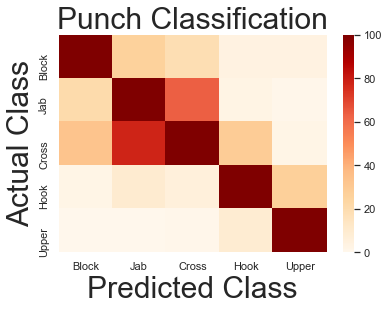
Jabs and crosses are misclassified as each other
Alright! So now we can see that Jabs and Crosses are the most likely confused. That's where a lot of our errors are coming from.
I proposed that rather than classifying 4 things with a moderate level of accuracy, we classify 3 things very well.
That means collapsing "Jabs" and "Crosses" into a single category: "Straight Punches".
Fortunately, this fits well into the general strategy of boxing. These punches have a natural association, and so replicating that association in our product will not be uncomfortable for our users.
What's our three-class accuracy?
We need to step back and replace our Jab and Cross categories with a Straight category.
#joining aggregate stats to previous df
sql_query = """
SELECT *,
CASE WHEN type = 'Jab' THEN 'Straight'
WHEN type = 'Cross' THEN 'Straight'
ELSE type END as new_type
FROM all_punches_sum_trans RIGHT JOIN puncher_info
ON file = filename
JOIN all_punches_sum_rot ON file = rotfile
"""
df=pd.read_sql_query(sql_query,engine)
#df[['type','new_type']]
# changed the label
y = df['new_type']
X = df[['sum_x_trans', 'sum_y_trans','sum_z_trans','sum_x_rot', 'sum_y_rot','sum_z_rot']]

# model remains the same
scores = cross_val_score(RandomForestClassifier(n_estimators=200, #the number of trees we'll be using
                                               min_samples_leaf=1, #the minimum size of leaf node
                                               max_features=4
                                                #the number of features considered for a split (out of six)
                                               ), X, y, scoring ='accuracy', cv=10)
scores.mean()
0.8557717620876317
Looks like a substantial improvement!
y_true = y_test
y_pred = model.predict(X_test)
mat = confusion_matrix(y_pred, y_true,labels=["Block","Straight","Hook","Upper"])
sns.set(font_scale=1)
sns.heatmap(mat, cmap='OrRd',
                vmax=100,
                xticklabels=("Block","Straight","Hook","Upper"),
                yticklabels=("Block","Straight","Hook","Upper")
           )

plt.title('Punch Classification', fontsize=30)
plt.ylabel('Actual Class', fontsize=30)
plt.xlabel('Predicted Class', fontsize=30)
<matplotlib.text.Text at 0x131bc7908>
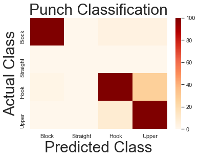
The only major errors are between hook and uppercut, and accuracy has increased from 77% to 85%. A lot closer to our goal of 1-1 responsiveness!
What I've demonstrated here is that while hyperparameter tuning can yield small improvements, sometimes the solution is to simplify the problem. I turned these results into my startup partners, and they proceeded to implement them in the product! I want to thank Insight and their partners for giving me this opportunity, and to thank you for reading!